
Here we’re quickly going to go through linear data structures. The thing that defines them is the order of things between structure elements. It’s defined as an abstract type independent from implementation. Examples (click to jump):
- Arrays
- Linked lists
- Stack (LIFO – Last in First Out)
- Queue (FIFO – First In First Out)
Frequent operations:
- element access
- search
- reading of writting
- inserts (all successing elements are being moved one place up)
- deleting (all successing elements are being moved one place down)
- finding a precursor and successor for an element
- list length
- merging two lists
- etc
There are numerous ways we can implement a linear list, as we mentioned in another post (Data structures), most frequent are sequential and linked lists.
Linear Data Structures: Arrays
This is the most basic and widely used type of data. It’s a homogenic structure with a finite number of elements. Efficient access (performance) with same physical & logical order of elements. The “disadvantage”, maybe aside from fixed size (memory space, max size), is that insert/delete operations can be costly.
Simplest one is a one-dimensional array or Vector. To define a place of an element (direct access), we’re using index (position).
Multi-dimensional arrays represent a generalization of one-dimensional ones. The two-dimensional array (or Matrix), can be considered as one-dimensional array containing one-dimensional arrays for elements.
Array Operations (representation, placement)
Basic one is a direct access using an array name and index value. Since we usually treat arrays as a sequential memory locations, inserting or deleting one element on a random location is inconvenient. Depending on the size, a lot of elements should be shifted (and indexes changed), thus performance might suffer.
As mentioned earlier (data structures, ), we can experience some issues if structures or elements sizes don’t take the same space as memory word size.
No filling:
|00000000|00001111|11112222|22223333|

Filling :
|00000000|0000----|11111111|1111----|

Padding:
|0000|0000|0000|1111|1111|2222|2222|3333|

* 0, 1, 2, 3 = elements
* - = padding/filling
If that happens, we have 3 options:
- no filling : Optimal space usage, but with the need to access and read multiple memory words, offsets, extractions, performance suffers
- filling : the remaining space in a last memory word is left unused. Space usage is not optimal but it’s more performant. We can calculate the usage as a relation between element size and space size reserved for it:
Su = s/⌈s⌉
If s>0.5, we rely on filling, if it’s <0.5, we’re turn to padding - padding : Placing a multiple elements in one memory word. If we have k elements in one memory word, usage:
Su = ks/⌈ks⌉wherek = ⌊1/s⌋
Here, the remainder until the next memory word is left empty.
Since the memory is a linear structure, vector is being placed naturally in it, but the matrix (X[1:M, 1:N]) has to be converted to a linear form. We can do this either by rows (C, Pascal) or by columns (FORTRAN). With rows, we’re going through column indexes first (N), then slowly shifting the rows index (M). With the column approach is the other way around M first, N second.
I don’t want to go into math details, but the way arrays are being placed can be useful. Although programmers can’t affect that, knowing how things work for a specific programming language can enable them to write more efficient code. There’s a great example of this below.
We’re doing matrix sums and each element can be placed in one memory word. Matrix is being placed in memory by rows. Cache memory of 256 memory words is being divided in 16 blocks of 16 words. First matrix element is mapped to a first word of the first block. Which one is more efficient?
SUM A:
sum=0
for i = 1 to 32 do
    for j = 1 to 16 do
        sum = sum + M[i,j]
    end_for
end_for

SUM B:
sum=0
for j = 1 to 16 do
    for i = 1 to 32 do
        sum = sum + M[i,j]
    end_for
end_for
Additional Placement Optimizations
On a matrix where significant amount of elements have 0 value we can do some optimizations. Two examples: triangular matrix and rare arrays/matrix.
Triangle matrix (X[1:n, 1:n]), where X[i,j] =0 for i<j (lower triangular) or i>j (upper triangular matrix). If we have <= or >= it’s strict lower and strict upper, respectively. We can save 50% of space.
Rare arrays/matrix, with high number of 0 valued elements (>80%). I didn’t use large matrix just for the purpose of e.g.:
    7 0 0
M = 0 2 9
    0 6 0
We can convert it to one record:
R   C   V
1   1   7
2   2   2
2   3   9
3   2   6
or 3 independent vectors:
R     C    V
1 ->  1 -> 7
2 ->  2 -> 2
      3 -> 9
3 ->  2 -> 6
Not ideal example, but you’ll get the picture. R holds the index of a column (C), and C holds the index of a V (non-zero values) Now we don’t have a direct access, but we do have a better space usage. On a large matrices that can be a significant save.
Linear Data Structures: Linked lists
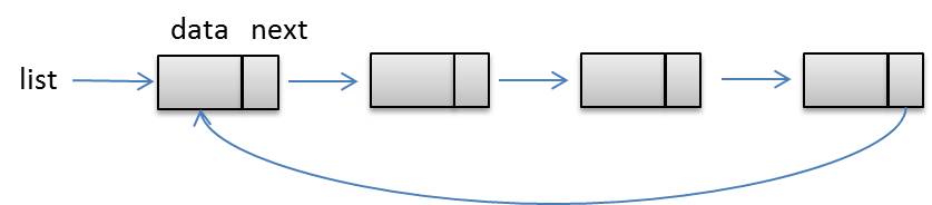
Linked lists remove some of the problems arrays have. The access is indirect, but the size is flexible/dynamic. Arrays have elements placed sequentially in memory. Linked lists can have elements placed anywhere in memory. Having that in mind, there must be a way to maintain the order of elements. This is achieved by placing the explicit address of a next element inside each of the elements. So, each element or node, aside from information contains a pointer (e.g. next). Access to the list is realised via one external pointer tied to the first node of the list (it’s not a part of the list). Empty list is null/nil (list=null). The basic example of singly linked list:
The list can be ordered or unordered (by some internal paramater/field). List that have elements pointing to both successor and predecessor are called double linked list. There are also circular linked list (successor of a last node is pointing to the the first node in the list).
Usually, lists are homogenic, but not exclusively.
Linked List Operations
Lists are generated dynamically and that requires some mechanisms to allocate and deallocate elements & space. There’s an approach to keep the free nodes and list nodes separated in individual lists. I guess it’s more perfomant, avoiding the cost of freeing and allocating memory all over again, but I’m not fully convinced that the gain is significant in general. Pseudo-code proved most useful when it comes to showing the algorithm principles :
GET_NODE:
if (avail = null) then
    ERROR
end_if
q = avail
avail = next(avail)
next(q) = nil
return q

FREE_NODE(p):
next(p) = avail
avail=p
Operations are mostly conducted through poitners, since they keep the list’s integrity.
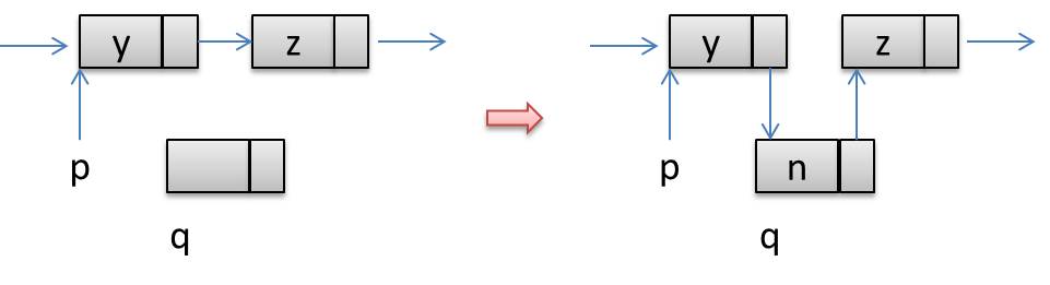
Linked list insert
Adding a node behind the specific node p:
INSERT_AFTER (p, new_data)
q = GETNODE
data(q) = new_data
next(q) = next(p)
next(p) = q
INSERT_BEFORE (p, new_data)
q = GETNODE
next(q) = next(p)
data(q) = data(p)
data(p) = new_data
next(p) = q
Linked list delete
DELETE_AFTER (p)
q = next(p)
next(p) = next(q)
FREENODE(q)
Delete first node:
DELETE (p)
q = next(p)
next(p) = next(q)
data(p) = data(q)
FREENODE(q)
Linked list search
Find the node with the specific content:
SEARCH (list, data)
p = list
while ( p != null) and (data(p) != data) do
       p = next(p)
end_while
return p
In an unordered list, we have to go through all of the elements. In an ordered one, we might consider some adjustments (data as an integer):
SEARCH_ORD (list, data)
p = list
while ( p != null ) and ( data(p) < data ) do
       p = next(p)
end_while
if ( p != null ) and ( data(p) > data ) then
      p = null
end_if
return p
Linked list invert
INVERTING (list)
p = list
q = null
while ( p != null ) do
     r = q
     q = p
     p = next(p)
     next(q) = r
end_while
list = q
Linked list concatenation
CONCATENATION ( list1, list2 )
if list1 = null then
     list1 = list2
     return
else if list2 = null then
     return
end_if
p = list1
while ( next(p) != null) do
     p = next(p)
end_while
next(p) = list2
Circular linked list insert
INSERT_AFTER_C (p, data)
q = GETNODE
data(q) = x
next(q) = next(p)
next(p) = q
if (list = p ) then
     list = q
end_if
Circular linked list concatenation
CONCATENATION_C ( list1, list2 )
if ( list1 = null ) then
     list1 = list2
     return
else if ( list2 = null ) then
     return
end_if
p = next(list1)
next(list1) = next(list2)
next(list2) = p
list1 = list2
Searching the circular list can lead us into infinite loop on unsuccessful search. Because of that we’re adding one pointer as the first node (heading), with some distinctive content/data that can’t be found on other “valid” nodes.
Inserting an node:
INSERT_C_H (list, data)
p = GETNODE
data(p) = data
next(p) = next(list)
next(list) = p
Double linked list
The disadvantage of circular list is that you have to go through entire list to get to the previous node. With double linked list offers a solution for that. Each node is tied to both precessor and successor nodes. It can have a header or be a circular one too. The operations are a bit more complex:
INSERT_AFTER_D (p, data)
q = GETNODE
data(q) = data
prev(data) = p
next(q) = r
next(p) = q
prev(r) = q
DELETE_D (p)
q = prev(p)
r = next(p)
next(q) = r
prev(r) = q
FREENODE(p)
Linked List vs Sequential Linked Lists
Although we need additional pointers in each node (using more space), it’s relatively small requirement. There are numerous examples of potential usages, for e.g. vector implementation of linked lists, rare arrays implemented via linked lists, set representations, polynome representation,etc.
Linear Data Structures: Stack
Stack is a dynamic (usually homogenous) structure and basically represent a type of linear lists with specific access type, adding/removing elements just from one end (LIFO – Last In First Out).
Bottom of the stack is fixed (bottom). Since only top of it moves, we need to keep track of it (stack pointer). Creating the stack S of maximum size n:
INIT_S (S, n)
ALLOCATE(S[1:n])
top[S] = 0
To check if a stack is empty:
STACK_EMPTY (S)
if ( top[S] = 0 ) then
     return true
else
     return false
Adding an element:
PUSH (S, data)
if ( top[S] = n ) then
    ERROR (Overflow)
else
    top[S] = top[S] + 1
    S[top[S]] = data
end_if
Removing top element:
POP (S)
if ( top[S] = 0 ) then
     return UNDERFLOW
else
    x = S[top[S]]
    top[S] = top[S] - 1
    return x
end_if
Fetch a TOP element only:
TOP (S)
 if ( top[S] = 0 ) then
     return UNDERFLOW
else
    return S[top[S]]
end_if
We can implement sequentially numerous stacks within one linear structure. As a simple example, we can have two stacks in one vector. First stack’s bottom is tied to the bottom of the vector (growing upwards) and the second stack’s bottom is tied to the vector’s top (growing downwards). We can have as many stacks as we can logically place in a vector. In one vector size of 20, we can place 5 stacks (size 4). We can optimize it further, for instance in situations where one stack (out of those 5) gets full, we can push the stacks in front of it (moving the elements upwards) to make space for additional element. I won’t write those operations/algorithms, but they’re out there.
Personally I wouldn’t want to complicate my life this way, but there is some logic to it. If we’re lacking the space, implementing multiple vectors independently would allocate twice the of memory. If those vectors (stacks) don’t grow as much, we could get a significant savings. Nowdays the memory is relatively cheap, but this might be handy (certain limits & conditions).
Stack Usages
Default example, cmopilers, OSs, arithmetic expression processing, processing subroutines.
Within aritmethical expressions, we have binary operators (operands on each side) and unary opeartor (operand in front/back). That’s a infix notation. It’s not quite suitable for compilers. In expressions with multiple operators and operands we can’t simply determine who belongs where. E.g. in A*B+C, is B an operand for * or +. We can use ( and ) to define it. Further on, to reduce number of parentheses, we can rely on operator prioritization.
To determine order of operator execution in subexpressions based on priority and level in an infix expressions requires out of compiler to go through it multiple times. That’s a main disadvantage of infix notation.
Further on, we can use Prefix and Postfix notation (operands in front, or in the back). A+B => +AB or AB+.
To convert an infix expression to postfix:
- place parenthesis
- move/replace right parenthesis with the operators,
- remove left parenthesis
Same thing for prefix (just inverted, towards left).
Calculating the expression in postfix notation:
EVAL_EXP ( postfix )
INIT_STACK(S, n)
while ( not_end_of postfix ) do
     x = INPUT ( postfix )
     if ( x = operand) than
         PUSH(S, x)
    else if ( x = un_op ) then
         oprnd = POP(S)
         res = x oprnd
         PUSH(S, res)
    else if ( x = bin_op ) then
         oprnd2 = POP(S)
         oprnd1 = POP(S)
end_while
res = POP(S)
if ( STACK-EMPTY(S) ) then
    return res
else
    ERROR ( INCORRECT EXPRESSION )
end_if
Algoritham example: A + B / C ^ 2 – E * F
7 + 8 / 2 ^ 3 – 1 * 2
X       operand1      operand2      res       S
7                                             7
8                                             7 8
2                                             7 8 2
3                                             7 8 2 3
^          2             3           8        7 8 8
/          8             8           1        7 1
+          7             1           8        8
1                                             8 1
2                                             8 1 2
*          1             2           2        8 2
-          8             2           6        6
So, the result of previous expression is 6.
Infix to Postfix Conversion
Efficient algorithm going through expression just once, linear complexity – O(n)
IN2POST (infix, postfix)
INIT_STACK (S, n)
rank = 0
next = INPUT(infix)
while (next) do
   if ( next = operand ) then
       OUTPUT (next, postfix)
       rank = rank + 1
   else
       while ( not ( STACK_EMPTY(S)) and (IPR(next) <= SPR (TOP(S)) )do
           x = POP(S)
           OUTPUT(x, postfix)
           rank = rank + R(x)
           if ( rank < 1 ) then
                ERROR (  INCORRECT EXPRESSION )
           end_if
       end_while
       if ( STACK_EMPTY (S) or ( next != ')' )) then
           PUSH(S, next)
       else
           x = POP(S)
      end_if
  end_if
  next = INPUT ( infix )
end_while
while ( not (STACK_EMTPY (S) ) ) do
    x = POP(S)
    OUTPUT (x, postfix)
    rank = rank + R(x)
end_while
if ( rank != 1 ) then
    ERROR ( INCORRECT EXPRESSION )
end_if
Since ther is no requirement to set parenthesis, we need to define priority.
oprator     ipr     spr      R
  +,-        2       2       -1
  *,/        3       3       -1
   ^         5       4       -1
   (         6       0       -
   )         1       0       -
IPR – moment it arrives on stack, SPR – already on stack
A + B * C – ( D + E – F ^ G ^ H) * ( I + ( J + K ) * L ) / M
next      S        postfix                   rank
A                  A                          1
+         +        A                          1
B         +        AB                         2
*         +*       AB                         2
C         +*       ABC                        3
-         -        ABC*+                      1
(         -(       ABC*+                      1
D         -(       ABC*+D                     2
+         -(+      ABC*+D                     2
E         -(+      ABC*+DE                    3
-         -(-      ABC*+DE+                   2
F         -(-      ABC*+DE+F                  3
^         -(-^     ABC*+DE+F                  3
G         -(-^     ABC*+DE+FG                 4
^         -(-^^    ABC*+DE+FG                 4
H         -(-^^    ABC*+DE+FGH                5
)         -        ABC*+DE+FGH^^-             2
*         -*       ABC*+DE+FGH^^-             2
...
For an expression: ABC * + D / , machine code equivalent (not optimal):
LOAD B
MUL C
STORE T1
LOAD A
ADD T1
STORE T2
LOAD T2
DIV D
STORE T3
Postfix notation is more appropriate for machine stack. Optimal:
PUSH A
PUSH B
PUSH C
MUL
ADD
PUSH D
DIV
Recursion..
Linear Data Structures: Queue
Similarly to stack, it’s a linear dynamic structure , but with two input/output points (front&back, FIFO – First In First Out). As with stack, it usually homogenous structure.
Sequential / Vector representation
Sequential representation is implicitly homogenous and limited in size. Two pointers, front and rear. One implementation that we can rely on is to move all elements down after each “delete” operation. More optimal approach is to wait for rear to meet the front of the vector. Even better implementation is circular buffer (empty: front = rear = 0). If front<rear, we’re getting the number of elements with: rear – front + 1. If front > rear, number of elements = n – front + rear + 1.
|   |   |   |   | 2 | 0 | 3 |   |
                  f       r
n=8, f=5, r=7 => front < rear => rear-front+1 => 7 - 5 + 1 => 3

 | 8 | 3 |   |   | 2 | 0 | 3 | 1 |
       r           f
n=8, f=5, r=2 => front > rear => n - front + rear + 1 => 8 - 5 + 2 + 1 => 6
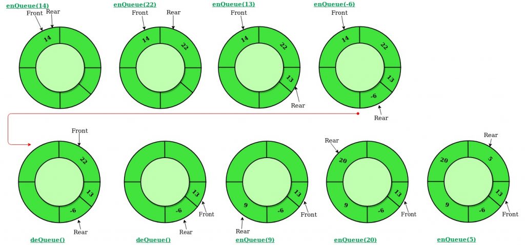
Usual operations: creation, inserts, deletions, reading and queue empty. Initialize queue (size of n):
INIT-QUEUE (Q,n)
  ALLOCATE Q([1:n])
  front[Q]=rear[Q] = 0
Insert operation first moves “rear” pointer to next element. If rear = front, queue is full, otherwise element is added. One specific situation is adding in an empty queue, when fron has to be set to 1.
INSERT (Q, p)
rear[Q] = rea[Q] mod n+1
if ( front[Q] == rear[Q] ) then
    ERROR ( Overflow )
else
    Q[rear[Q]]=p
    if ( front[Q] == 0 ) then
        front[Q] = 1
    end_if
end_if
For deletion, we’re first checking if the queue is empty (front == 0). If not, we’re returning the element and moving the front upwards. if (front == rear) we’re setting them to 0.
DELETE (Q)
if ( front[Q] == 0 ) then
    return ERROR (underflow)
else
    e = Q[front[Q]]
    if ( front[Q] = rear[Q] ) then
        front[Q] = rear[Q] = 0
    else
        front[Q] = front[Q] mod n + 1
    end_if
    return e
end_if
Checking if queue is empty:
QUEUE_EMPTY (Q)
if ( front[Q] == 0 ) then
    return true
else
    return false
end_if
Getting the front element without removal:
FRONT (Q) :
if ( front[Q] == 0 ) then
    return ERROR (underflow)
else
    return Q[front[Q]]
end_if
QUEUE_EMPTY-1 (Q):
if ( front[Q] == rear[Q] ) then
    return true
else
    return false
end_if
DELETE_1 (Q):
if ( front[Q] == rear[Q] ) then
    return ERROR (underflow)
else
    front[Q] = ( front[Q] + 1 ) mod n
    return Q[front[Q]]
end_if
There’s one disadvantage again. If queue gets full, front=rear, we’re ending up with the empty queue being equal to the full one. To circumvent this, we’re not allowing the queue to have more than n-1 elements. Full queue: front=(rear+1) mod n
INSERT_1 (Q, x):
rear[Q] = ( rear[Q] + 1) mod n
if ( front[Q] = rear[Q]) then
    ERROR (overflow)
else
    Q[rear[Q]] = x
end_if
Double Ended Queue
Inserts and deletions are conducted from the both ends. Front and rear lose meaning. There are a couple of variants: no restrictions, input-restricted deque (one insert side) and output-restricted deque (one deletion side).
Linked list queue
Outer pointer, first element, points to the list (front). Last element basically points to rear. Insert operation creates new node, rear pointer next value points to it and we reassign rear pointer to new node.
INSERT_L (q, x):
p = GETNODE
info(p) = x
next(p) = nil
if ( rear[q] == nil ) then
    q=p
else
    next ( rear[q] ) = p
end_if
rear[q] = p
Deletion removes an element and reassigns the pointer(s):
DELETE_L (q)
if ( q == nil ) then
     ERROR (underflow)
else
    p = q
    x = info(p)
    q = next(p)
    if ( q = nil ) then
        rear[q] = nil
    end_if
    FREENODE(p)
    return x
end_if
Priority Queue
This is the structure in which order of elements (by content, by value) has a decisive factor on which element is going to be removed. It’s necessary to have a value/field (or a number of them) on which elements can be compared. This defines the “priority” of elements. Two types of priority queues:
- max priority
- Inserts are random, but on deletion always the minimum valued element is being removed
- min priority
- Inserts are random, but on deletion always the maximum values element is being removed
As for the implementation, different types, different efficiencies, linear structures, sequential or linked list.
Conclusion
Linear data structures are building blocks of everything, weather you use them in their raw form, library, on some distributed system (semaphores) or in your buffer overflow reverse engineering stuff, they’re unavoidable segment of computing. This was a rough walkthrough, mixing little bit of everything. It was mostly theory (not including pseudocode) but we’ll most likely get back to this at some point later on, adding practical examples in C/C++ or Java.


